Encoding In Language

27 Jan 2023 - Ryan Llamas

“Almost every problem that you come across is befuddled with all kinds of extraneous data of one sort or another; and if you can bring this problem down into the main issues, you can see more clearly what you’re trying to do and perhaps find a solution.”
— Claude Shannon

Probability In NLP

Language is unpredictable and can change so often that is seems impossible for a machine to produce words or phrases like us. But through probability, one could measure the relationship of words, sentences, paragraphs, and more to measure predictability in a word set to see the connection that form between them.

But how is probability used in language? Let’s break this down piece by piece. By definition, the act of probability is “the extent to which something is probable; the likelihood of something happening or being the case.” But how does one end up measuring something that could likely happen. It all starts to man’s basic ability, counting. Counting is a simple procedure, and can give us loads of information. Let’s take the example of a coin flip. Given a coin has heads and tails, you could keep flipping it to find a relatively even distribution of heads and tails. You could then make the argument that you have a “fair” coin.

But what about language? Language is after all much more chaotic and free vs. the limitations of simply flipping a coin. There are more variables to consider, such as how often: a word is used with another, a word used in a particular section of time or place, a collocation or phrase is uttered at a given event, etc. The list could go on and on if you put your mind to it, and you’ll find the use case that is aimed to be measured can yield interesting findings.

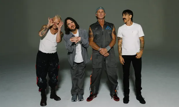
To draw associations between one event with another, you need to count distributions of data and track when one event overlaps with another. Let’s create a fun example for the sake of entertainment and learning. Let’s say I started to track how often band members are mentioned in two entertainment articles. Let’s say the band is Red Hot Chili Peppers to throw some more fun into the problem (guilty, I am a fan).

In the articles, I find:

Article#1 mentioned band member:

Anthony Kiedis: 7 times
Chad Smith: 0 times
John Frusciante: 2 times
Flea: 5 times

Article#2 mentioned band member:

Anthony Kiedis: 4 times
Chad Smith: 1 times
John Frusciante: 0 times
Flea: 7 times

By simply counting the names of these band members in both articles, I could then map out a probability space and find associations between the band members. In this case, I want to find the probability of finding Anthony Kiedis in both articles if I were to try and find a random band member’s name.

The probability of me finding Anthony in Article#1 comes up as \(\frac{1}{2}\), while for Article#2, I find Anthony \(\frac{1}{3}\) of the time. To find the probability of finding Anthony in both articles out of all names requires us to find the joint distribution. This is defined as:

\[p(x, y) = p(x) \times p(y)\]

In our case, the probability of finding Anthony in both articles by choosing the first random band member name I find is

\[p(\text{Anthony In Article#1, Anthony in Article#2}) = \frac{1}{2} \times \frac{1}{3} = \frac{1}{6} = 16.6667\%\]

But let’s say I wanted to know the relationship between band members in these articles, such that I wanted to see how often a band member’s name occurred given another band member is mentioned. A use case for this is possibly to see how often a pair of band members is considered a good pair by the media. In this case, I would be calculating the conditional distribution. This is defined as:

\[p(x\mid y) = \frac{p(x,y)}{ p_{Y}(y) }\]

Another way of looking at \(p(x\mid y)\) is what is the probability of x given y is already known. But wait, what is then \(p_{Y}(y)\)? This is called the marginal distribution. This is defined as:

\[p_{Y}(y) = \sum_{x} p(x,y)\]

Think of this as totalling up the probabilities of the event y happening with each event x. After all, to truly know the relationship of these two values, we have to know how y behaves for every instance of x, to truly understand how much of a dependence it has on y. You could also apply the opposite logic to x with \(p_{X}(x)\).

Now, back to our example. One thing to note about conditional distributions, they work best when a set of events are neither independent nor mutually exclusive. I couldn’t for example, try to find the probability of finding Anthony’s name in both articles given I know the probability of finding Flea’s name is in both articles. Both are independent events because one as no influence over the other, and vice versa. Such that:

\[p(\text{Anthony In Article#1&2}\mid \text{Flea In Article#1&2}) = p(\text{Anthony In Article#1&2})\] \[p(\text{Flea In Article#1&2}\mid \text{Anthony In Article#1&2}) = p(\text{Flea In Article#1&2})\]

Another puzzling piece, I need to find a way to group these events with a limited subset of data. I couldn’t group it by article because I am currently guaranteed to find Anthony and Flea mentioned in both articles, such that:

\[p(\text{Anthony In an Article}\mid \text{Flea In an Article}) = 1\] \[p(\text{Flea In an Article}\mid \text{Anthony In an Article}) = 1\]

Maybe if I had 100 or 1000 articles, I am bound to find some that mention only Flea and some that only mention Anthony. But even then, am I truly solving the problem of finding relations between band members? What if Flea was only mentioned once when Anthony was mentioned several times in a given article? It wouldn’t be fair to say then that the article identifies Flea and Anthony as having a relation. In this case, it’s a matter of grouping your data in such a way that allows you to still solve the problem. So, lets group the data from articles to sentences. Such that:

Article #1&2 sentences with mentioned band member:

Anthony and Chad mentioned in a sentence: 2
Anthony and John mentioned in a sentence: 0
Anthony and Flea mentioned in a sentence: 3
Chad and John mentioned in a sentence: 0
Chad and Flea mentioned in a sentence: 0
John and Flea mentioned in a sentence: 1

Now we’re talking. By grouping the data to lower groupings, we can now start to see relationships form in the text. We could even go further with these groupings by splitting words into small groups versus sentences and counting the times we see these two events. But for the sake of a simple (as it can be) example, let’s see what the conditional distributions are:

\[= p(\text{Anthony is in the sentence}\mid \text{Flea is in the sentence}) \\ \implies\frac{\text{Probability of Anthony and Flea mentioned in a sentence}} {\text{Marginal Distribution of Flea with each band member}} \\ \implies\frac{3}{4} = 75\%\]

And

\[= p(\text{Flea is in the sentence}\mid \text{Anthony is in the sentence}) \\ \implies\frac{\text{Probability of Anthony and Flea mentioned in a sentence}} {\text{Marginal Distribution of Anthony with each band member}} \\ \implies\frac{3}{5} = 60\%\]

With this information, I can then say that Flea has a strong dependence with Anthony, while Anthony can be paired with other band members and still have a relevant presence. This sort of information can tell a lot given the proper use case, and can even be used to build complex algorithms to estimate surprise and compress information. This is where information theory comes into play.

Information Theory in Language

Information Theory is the ability to communicate information from one source to another with minimal interruption and loss of information given that noise (the interference between the source and destination) is present in your process. We can thank the work of Claude Shannon for this field, as his original paper A Mathematical Theory of Communication gave rise to many methods of estimation and NLP models that persist to this day. I couldn’t help but take time to read a good portion of this paper, as I wanted to see the foundations that created an entirely new field during his time.

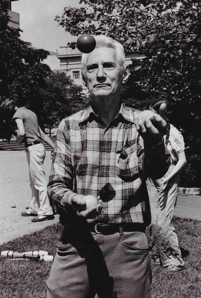
Picture of Claude Shannon Juggling

Claude Shannon is an individual that couldn’t possibly be ignored. He was a student of MIT contributing to many fields such as Boolean algebra and Cryptography. His playful nature could be shown too, as he would make many fun contraptions at Bell Labs like juggling machines and robotic turtles. But this playful nature did not sidetrack him from the main problems he was aiming to solve. His collages referred to him as someone who takes on the hard problems because they were hard by nature. I think we can all learn a thing from Shannon in the perseverance of seeking knowledge when the road is wrapped in a veil.

But what did Claude Shannon discover in his paper? His findings showed that you could make a model that could minimize the loss of information and estimate the amount of surprise for a given set of symbols. He also coined the term “bit” in this paper, as he would convert his symbols into 0’s and 1’s based on their predictability. But just how is the value of surprise defined for a given set of symbols? This is through entropy, which is defined as:

\[H(X) = - \sum_{x \in X} p(x) \log_{2}p(x)\]

Shannon defines entropy in the paper as “playing a central role in information theory as measures of information, choice, and uncertainty”. But how does this evaluate surprise of a symbol? With \(-\log_{2}p(x)\), we are able to determine how much surprise we expect for one given symbol with a base of 2, which translates to the size of a bit (0 or 1). For example, consider a fair coin is flipped. The amount of bits represented for heads being up translates as:

\[-\log_{2}p(1/2) = 1 \text{ bit}\]

Multiplying \(p(x)\) allows us to see the probability of this bit appearing. If we were to apply this back to the previous example, we would find:

\[1/2\times-\log_{2}p(1/2) = 1/2\]

This means heads alone would take up half a bit, such as only being 0 or 1 in this case. By taking the sum (\(\sum\)), then we are able to determine the average amount of bits for a coin flip, which becomes our entropy value. Such that:

\[H(X) = - \sum_{x \in X} p(x) \log_{2}p(x) \implies p(1/2)\log_{2}p(1/2)+p(1/2)\log_{2}p(1/2) \\ \implies \text{Average of 1 Bit for a coin flip}\]

We can say now an average of 1 bit is expected for a coin flip. This is a telling sign that there will be little surprise and information when encoding this.

As the probability of a set of outcomes becomes more sparse and even, more information can be expected. Consider the scenario of a local town having ten events, each having a 10% chance of occurring each year. Calculating the entropy for those events yield:

\[H(X) = - \sum_{x \in X} p(x) \log_{2}p(x) \implies 10 \times (p(1/10)\log_{2}p(1/10)) \\ \implies \text{Average of 3.321928094887362 Bits for an event in a given year}\]

Considering each event has an equal probability of occurring in great numbers, the amount of information expected increases as well!

Now, how can this be applied to language? When applied, you can determine the amount of information for a single word or collocation. This also means you can reduce the amount of information needed to communicate the proper intention.

For example, lets say I was an explorer of sorts and wanted to let people know what city I am in. There are a tons of cities in the world, each with a vibrant name. I could be in Chicago, New York, or Krungthepmahanakhon Amonrattanakosin Mahintharayutthaya Mahadilokphop Noppharatratchathaniburirom Udomratchaniwetmahasathan Amonphimanawatansathit Sakkathattiyawitsanukamprasit (Yes, this is a real city name!).

Also referred to as the city of Bangkok!

But when I factor in the probability of the explorer being in a city and apply bits in my communication, then I can reduce this information dramatically. Krungthepmahanakhon Amonrattanakosin… (you get the point) now becomes a collection of 0’s and 1’s to effectively communicate where I am. This could do wonders in saving performance in systems that handle large amounts of text that have recurring themes. It can also define the amount of information associated with a city for the given use case, defining the amount of surprise when a city is listed.

But how is language effectively translated to 0’s and 1’s? While entropy can certainly be a useful method to evaluate surprise, it would be hard to ignore just how it is translated to 0’s and 1’s. This is where encoding comes into play.

Encoding and Decoding Information to Bits

While reading Foundations of Statistical Natural Language Processing, 1st Edition, my eyes were caught by the bottom highlighted section below:

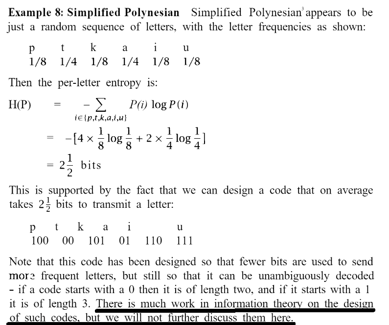
“What!? Why wouldn’t we explore how these codes are generated!” I exclaimed after seeing this sentence. This is such a cool tool that can’t possibly be ignored, and I had to explore it. You could say I went on a tangent with information theory and language, as I was shying away from entropy and digging into encoding algorithms.

Nonetheless, entropy and the encodings do have some correlation, as mentioned in the passage shared. When entropy is evaluated, the average amount of bits needed becomes apparent as well when encoding the symbols. This can be an indicator on how much information will be generated when compressing this info.

But what entropy encoding algorithms exist to evaluate these group of bits you may ask? There exist so many! Here are a few examples:

Huffman Coding
Unary Coding
Arithmetic Coding
Shannon-Fano Coding
Elias Gamma Coding
Tunstall Coding

We haven’t even listed them all which is the beauty of these algorithms. Each serve a distinct purpose and use case all because there is not a one-size fits all solution. Instead, it is a wealth of tools available for use, and knowing which one to use is half the battle.

For example, take the difference between Shannon-Fano and Huffman coding (we will mainly be discussing these two algorithms for now in the duration of this post). Huffman coding can produce variable length encodings such that a set of codes could be 10, 11, 100 with various bit sizes vs. Shannon Fano coding which produces fixed length encodings such as 100, 110, 111 where the bit size is always three. This can greatly effect the length of your compression depending on the probability set’s distribution.

These algorithms do wonders by taking data and shrinking it in size (hence compression). Let’s take the above passage from the book as an example:

1000010101111100010101110 100 00 101 01 111 100 01 01 01 110 p t k a u p a a a i

Notice how I am able to decipher this set of bits with minimal interruption (other than me manually eyeing the key and the code to ensure they are correct for this example). I am able to parse through these bits and find a set of symbols simply by looking left to right with the bit stack and splitting when a set is found in the key. That is the benefit of these algorithms, the ability to encode the keys without hindering the ability to decode them. Note however these encodings do not work with the presence of noise in your system, such that by inserting an extra bit will still generate a valid code, but give a completely new set:

100001010111

1100010101110 100 00 101 01 11

110 00 101 01 110 p t k a u a t k a i

Now that we know how to decode a set of bits, your probably wondering how we go about encoding it. Both Shannon and Huffman coding algorithms relies on probability. In particular, the individual probability of a set of symbols. With the probability of each symbol, we can then build a binary tree that maps out our bits. But how we go about building that tree is what separates these two algorithms. Let’s start with Shannon Fano encoding and use the example in the passage. The pseudocode is defined:

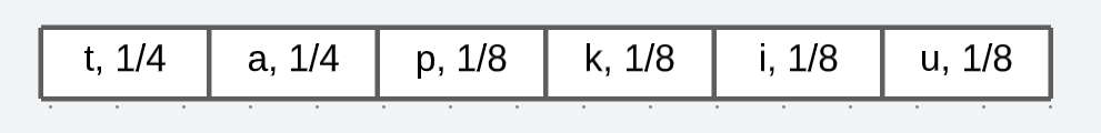
Organize the probabilities with its associated symbol in sorted descending order
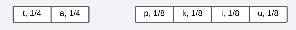
Split the symbols down the middle where each sets total probability sum has a small difference (Such that 50-50 is preferable over 25-75)
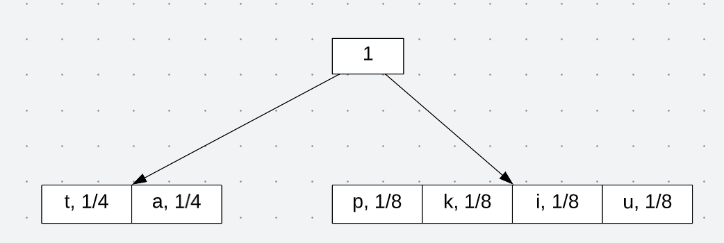
Reference back to the total probability value of the original list (Should end up to be 100% for the first time around)
Perform Step 2-4 again for each set until you end up with leaf nodes that contain one value
Assign the least probable (left) references with 0 and most probable (right) references with 1 for the entire tree

Let’s see this in action. First, the organized probabilities with its symbol in descending order:

Now we split the array based on how close the probabilities are to one another. In this case, we get a nice 50-50 split:

And reference it back to its total probability:

Now perform the same steps with each set. It should look like:

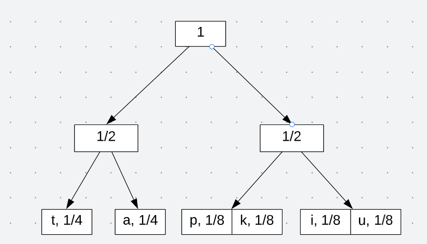
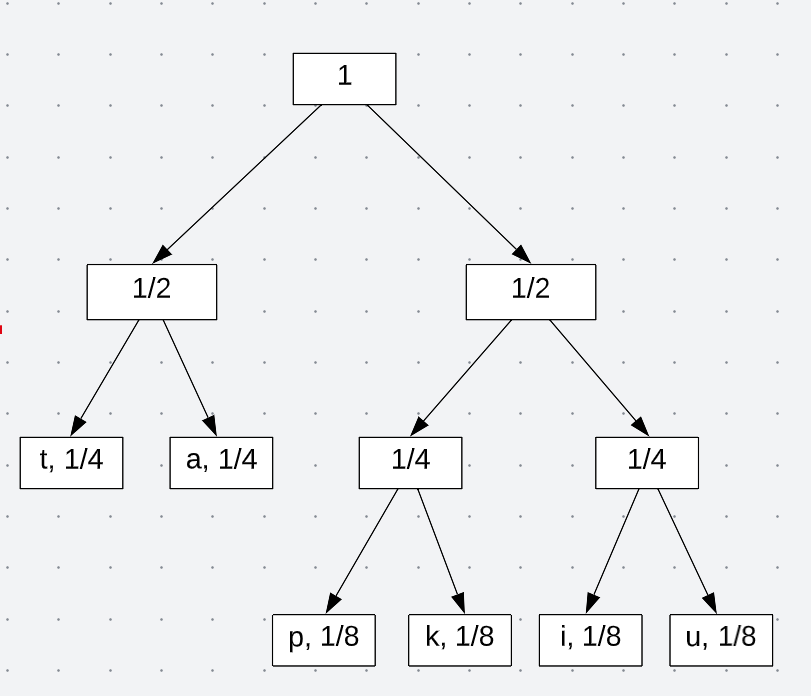
Now that we have leaf nodes with one value/symbol, we can then assign bits based on its probability:

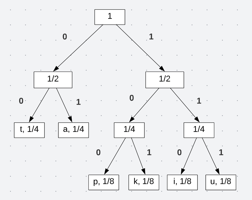
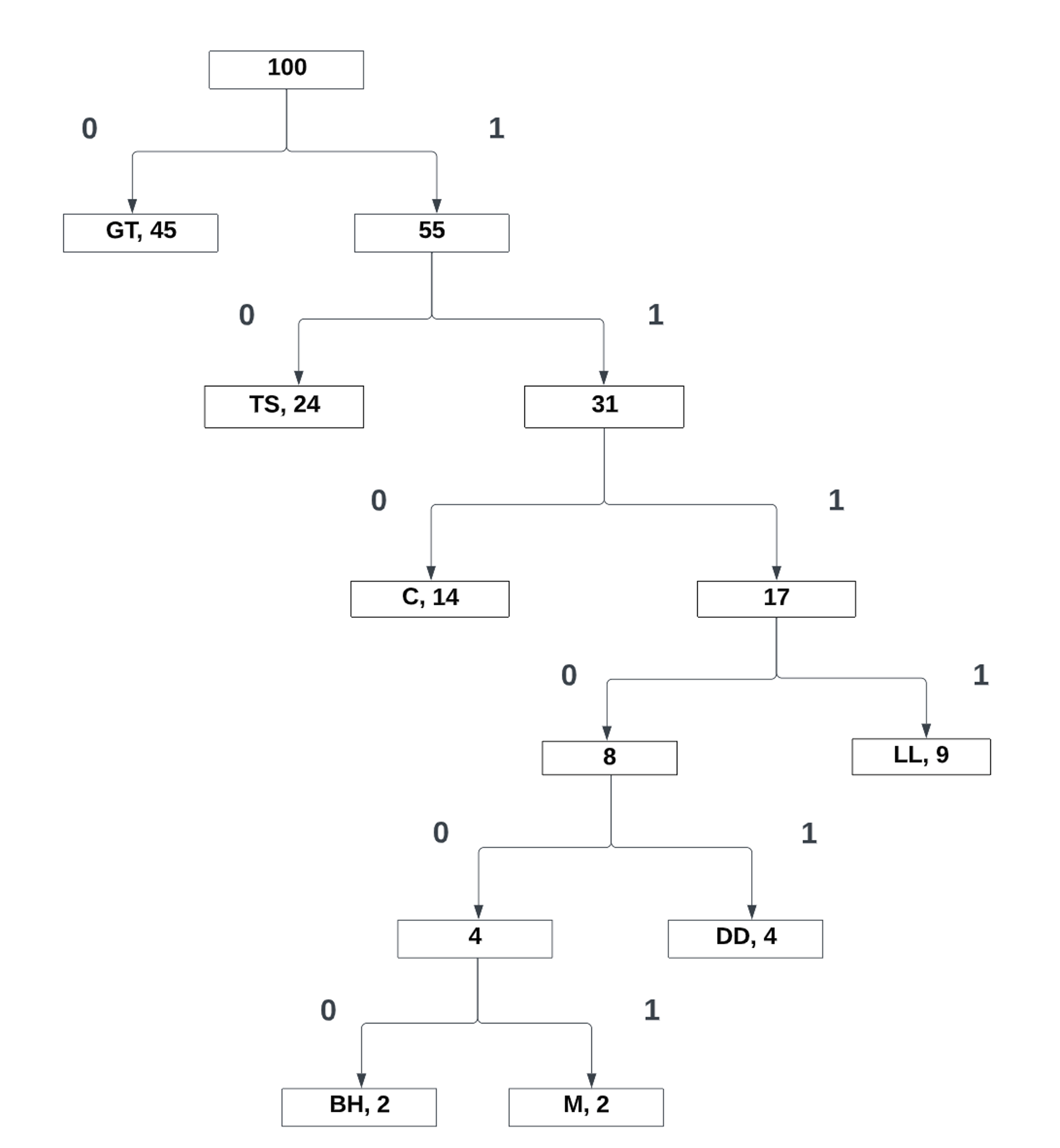
With this tree, by traveling from the root to the leaf node, I am then able to define encodings for each symbol. Take the letter “k” as an example. Traveling down the tree yields the following encoding:

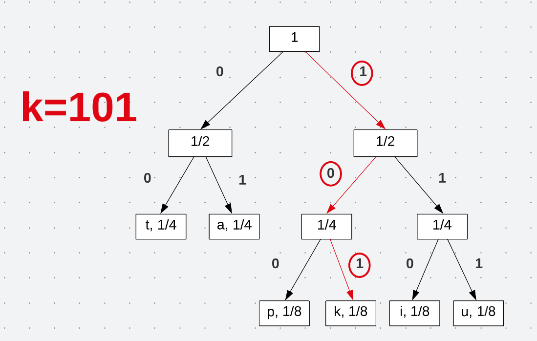
See how traveling down to each node leads to a new encoding. Starting at the root, I am able to define a unique encoding that can be used to communicate a message. All the encodings end up being exactly how we found in the passage:

\[t = 00 \\ a = 01 \\ p = 100 \\ k = 101 \\ i = 110 \\ u = 111\]

Now I can effectively communicate a message with minimal loss of information. But maybe I don’t want to use fixed length encoding, but instead, I wish the length to vary in size. Better yet, I want to have a coded solution on hand. This is where Huffman Encoding comes into play.

Entropy and Huffman Encoding Code Challenge

For this posts coding challenge, I decided to code a solution for Huffman coding and calculate the entropy value based on the words being analyzed. This will involve parsing through a text document, counting words that are to be measured, encoding the given words with Huffman, and then calculating the entropy value for the given set.

Before we do that, lets discuss on how Huffman coding works. Unlike Shannon-Fano encoding, Huffman coding uses variable length encodings. This means the length of the encodings can vary in bit size. Such that a high probability symbol may produce “1”, but the lowest probability symbol could expand out to 100101001… Of course, this depends on just how many symbols/words you identified in your set.

The pseudocode for Huffman Encoding is as follows:

Take the two lowest probabilities in your list
Reference back these probabilities to a total sum
Remove the two lowest probabilities and push the new total sum to the list
Perform Steps 1-3 until you end up with one probability value as the root
Assign 0 to the left reference and 1 to the right reference

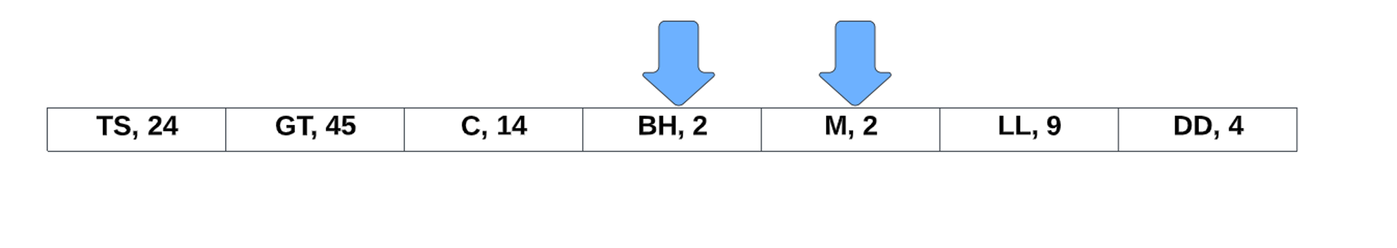
Let’s go through an example. Let’s say I was analyzing a book to determine what location is often used in the text. Let’s say this book is The Hobbit by J.R.R. Tolkien. After performing a count, there are 7 distinct locations used:

The Shire(TS)
: 24%
Goblin Town(GT)
: 45%
Carrock(C)
: 14%
Beorn's Hall(BH)
: 2%
Mirkwood(M)
: 2%
Long Lake(LL)
: 9%
Desolation of the Dragon(DD)
: 4%

(Note: This is very much dummy data and not measured. Although, I am curious to find a way to measure where someone is in the text based on context clues. Something to look into in the future)

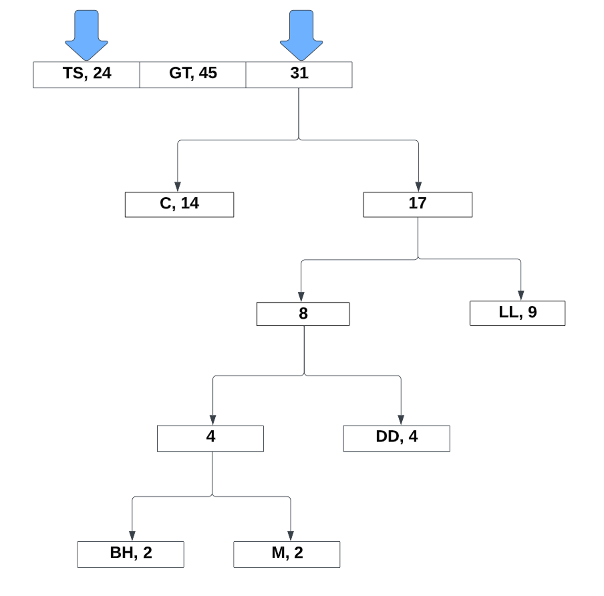
Now, lets put this pseudocode code in action. First, we need our probability list:

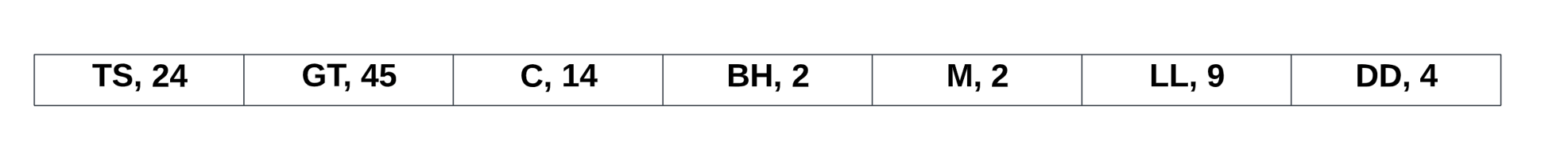
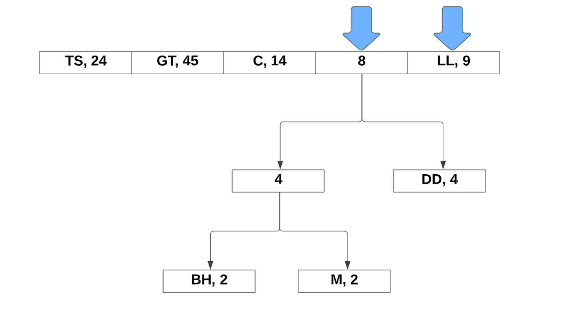
Notice how it is completely unordered. Unlike Shannon Fano coding, the Huffman coding can still function regardless of the order. Now, lets take the two lowest probabilities and make a reference to its total:

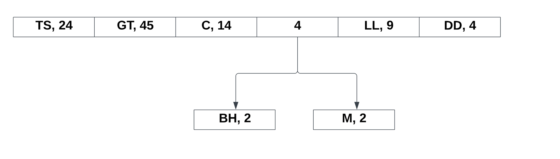
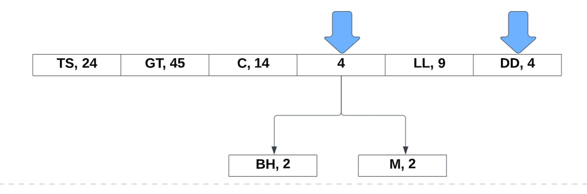
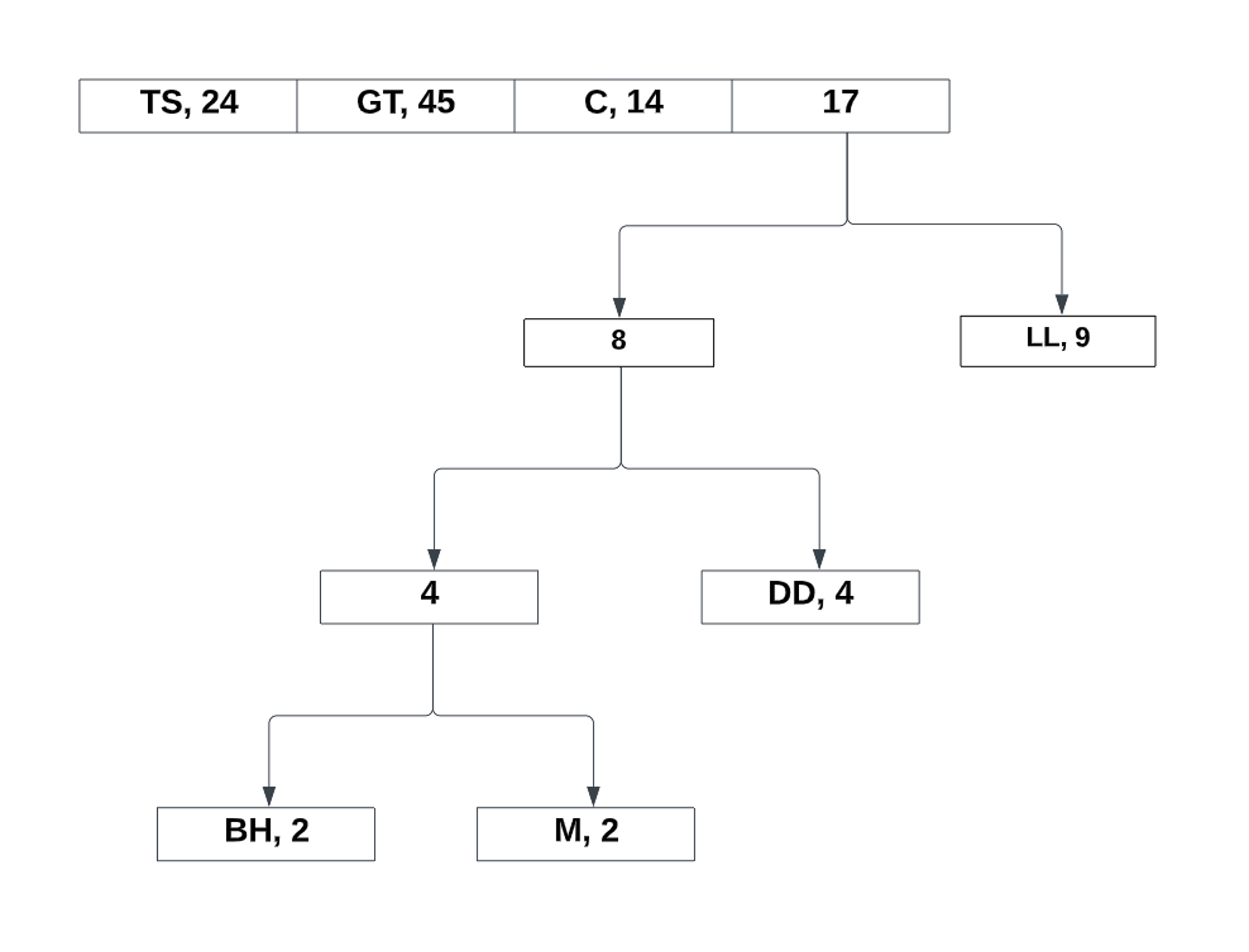
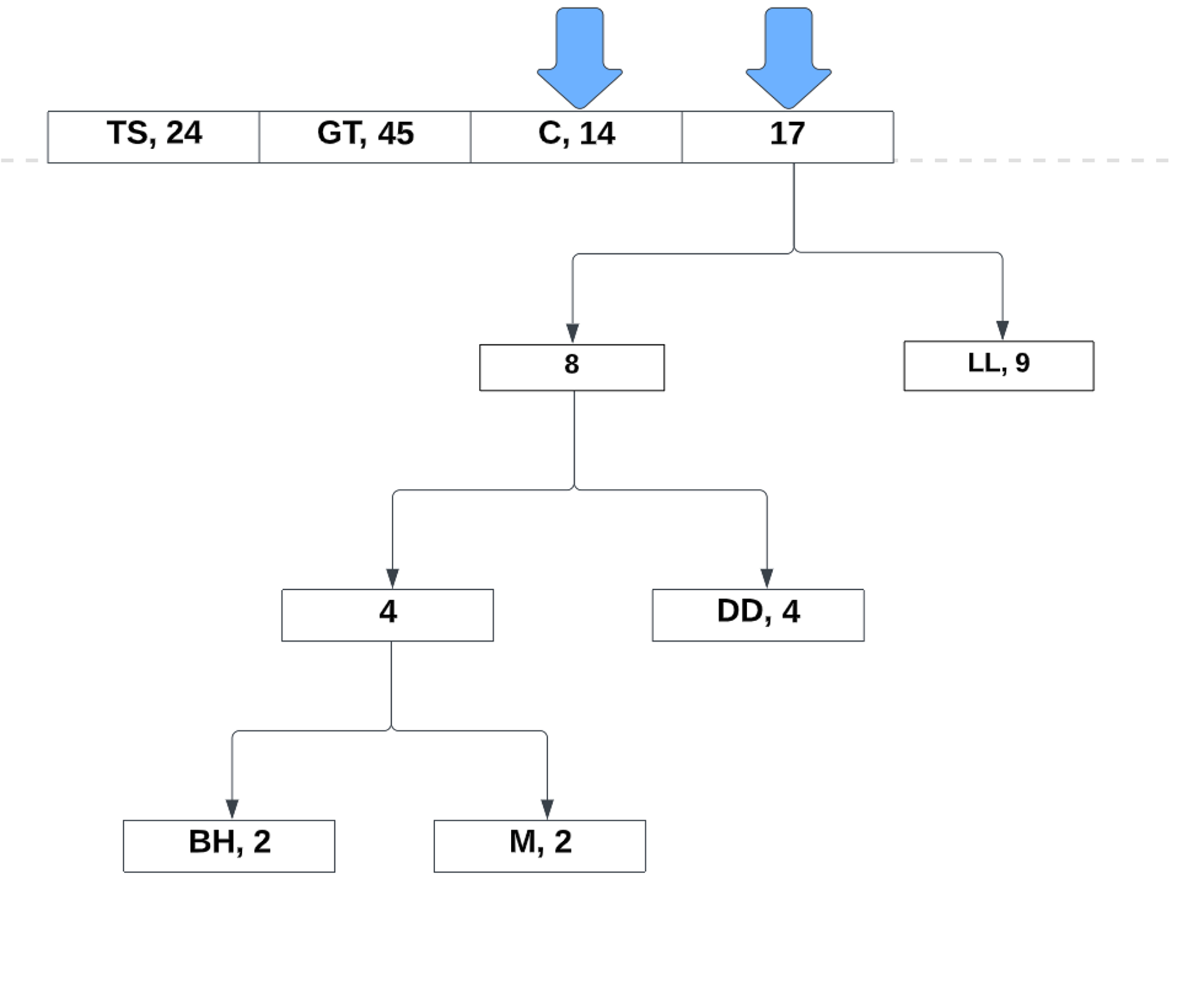
Now the new values takes its place in the list. From there, we continue to repeat the process:

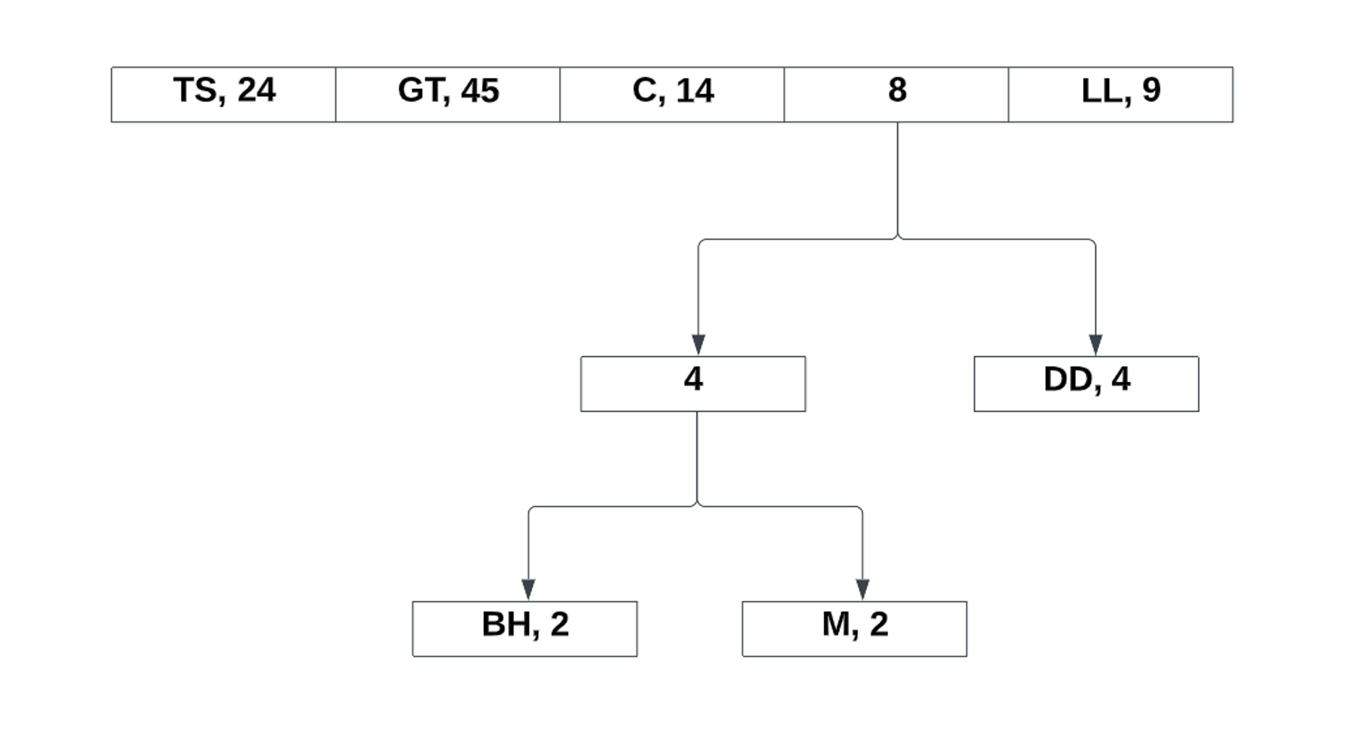
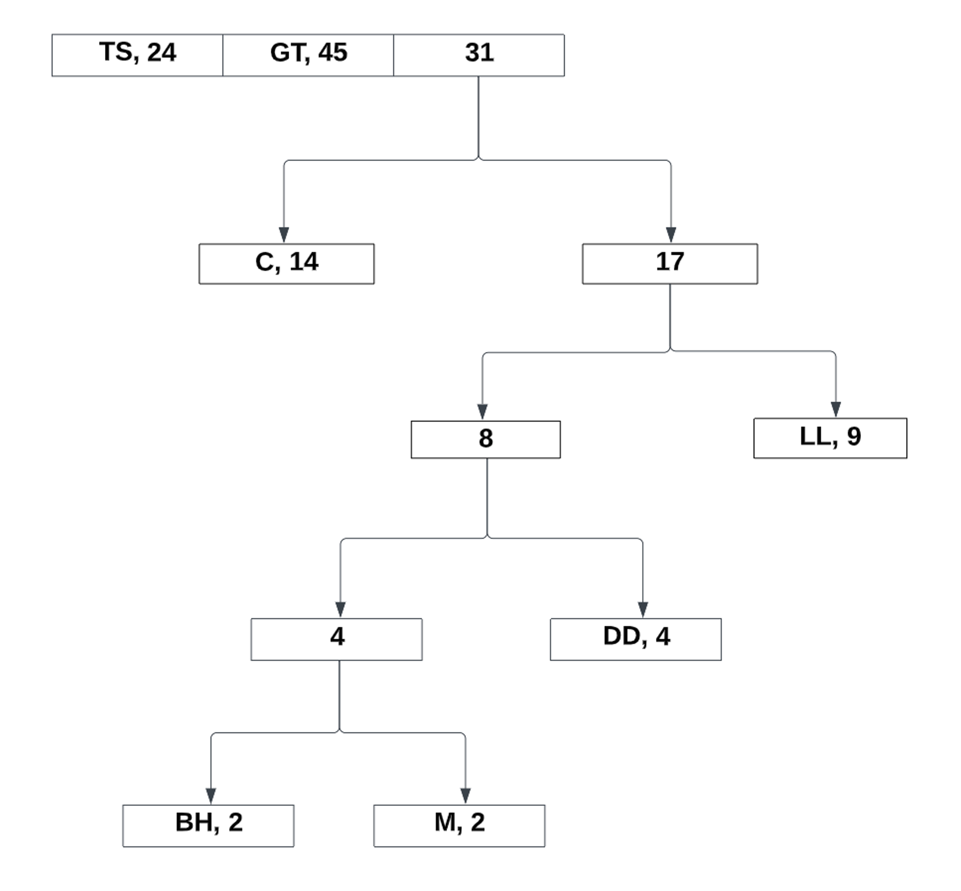
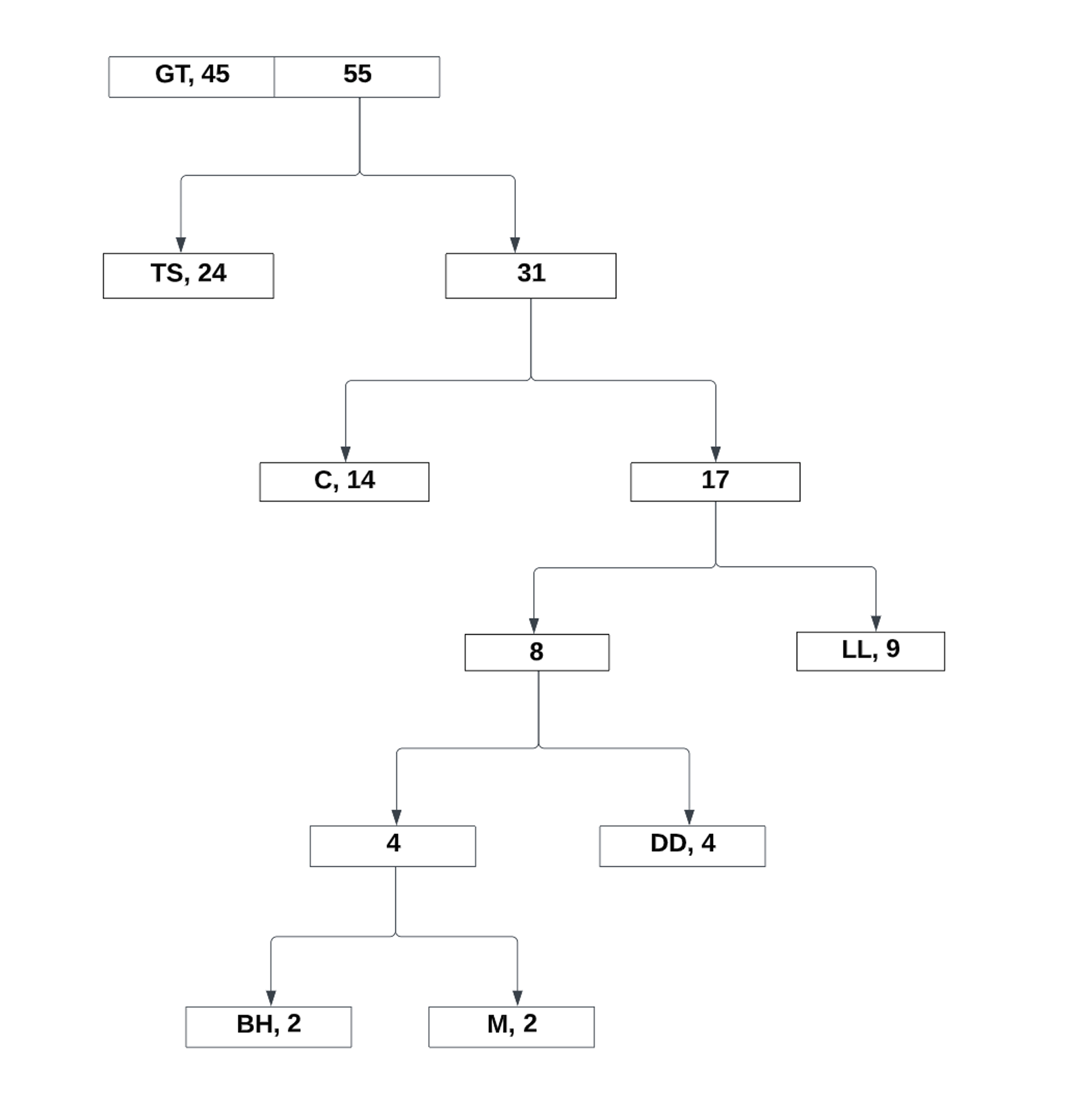
After the last two values, all that is left to do is assign the bits to the left and right references:

Now that we know how huffman encoding works, let’s jump back into the coding project. Deciding on what to use as a dataset to create these encodings was certainly a challenge. I knew I wanted to use something fun, so I eventually landed on the idea to look at a popular book. The book series I eventually went with was Harry Potter

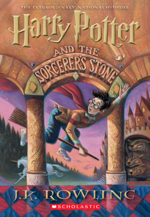
But what to encode? I needed a common subject to look at that could be effectively counted without too much complexity. Locations, moods, and colors came to mind, but I eventually decided to go with names (similar to what I did for the Red Hot Chili Peppers example). This proved to be interesting as I had to do research into some popular characters for the series and come up with a list of names to search for.

After about four working days looking at this problem, I eventually came to a solution. I like to think my python coding and test case implementation has improved after this challenge. But it will only get better after I complete more challenges that relate to NLP.

Coding Solution

For the names I am searching for, I made a text file with some pretty popular characters in the series. You’ll find I excluded the most popular character Harry. There is a good reason for this. His name was used so often (as expected) that is ended up being about 50% of all names in the books. Removing his name, the data set was more interesting to examine because it became evenly distributed (or as close as it could be).

Voldemort
Ron
Hermione
Ginny
Draco
Neville
Rubeus
Minerva
Severus
...

But now where do I get the books? It turns out there are git repos available that house the text versions of the books free for use. Not only did I use one of these books, but I decided to use two. This allowed me to test my code with another word set to examine and account for edge cases, such as a character existing in one book, but not the other.

Let’s take a look at main() to see how the execution of this project is structured

1
2
3
4
5
6
7
8
9
10
11
12
13
14
15
16
17
...

def main():
    print("******************************* Philosophers Stone Data *******************************")
    frequencyDistTrackerForPhilosopherStone = get_frequency_dist_tracker(tokenize_harry_potter_book_philosopher_stone())
    print("Entropy of characters from \"Philosophers Stone\": " + str(entropy(frequencyDistTrackerForPhilosopherStone)))
    graph_frequency_dist(frequencyDistTrackerForPhilosopherStone)
    perform_huffman_coding(frequencyDistTrackerForPhilosopherStone)

    print("\n******************************* Chamber of Secrets Data *******************************")
    frequencyDistTrackerForChamberOfSecrets = get_frequency_dist_tracker(
        tokenize_harry_potter_book_chamber_of_secrets())
    print("Entropy of characters from \"Chamber of Secrets\": " + str(entropy(frequencyDistTrackerForChamberOfSecrets)))
    graph_frequency_dist(frequencyDistTrackerForChamberOfSecrets)
    perform_huffman_coding(frequencyDistTrackerForChamberOfSecrets)

...

There are three parts to this program. First is get_frequency_dist_tracker(...) which counts the names being searched in the book text, the book text being in this case tokenize_harry_potter_book_philosopher_stone(). After it counts the amount of times a name has appeared in the text and returns its probability, it will be saved in a variable like frequencyDistTrackerForPhilosopherStone.

I go ahead and then calculate the entropy value for this distribution by directly printing it with str(entropy(...)). This gives a good indicator of how many bits on average is used for a given set of symbols.

After the entropy value is printed, I decided to do a little exploring with graphing in python, as presenting your data in a visual manner is important. The method call graph_frequency_dist(...) and perform_huffman_coding(...) does this, as it will print a bar graph of the distribution of names and a visual binary tree of the huffman encoding graph. Of course, perform_huffman_coding(...) does more than graph the binary tree, as it will also perform the algorithm to build the huffman tree as well.

Let’s go ahead and take a look at how the program goes ahead and tokenizes the book content with method tokenize_harry_potter_book_philosopher_stone()

1
2
3
4
5
6
7
8
9
10
11
12
13
14
...

def tokenize_harry_potter_book_philosopher_stone():
    url = "https://raw.githubusercontent.com/formcept/whiteboard/master/nbviewer/notebooks/data/harrypotter/Book%201" \
    "%20-%20The%20Philosopher's%20Stone.txt"
    bookText = requests.get(url).text

    removePunctuationTokenizer = nltk.tokenize.RegexpTokenizer(r'\w+')
    bookTextPunctuationRemoved = removePunctuationTokenizer.tokenize(bookText)

    getCharacterNamesTokenizer = nltk.tokenize.RegexpTokenizer(get_regex_for_all_characters())
    return getCharacterNamesTokenizer.tokenize(' '.join(bookTextPunctuationRemoved))

...

Here I reference the content of the book with an url to a raw text link and make a http request to get it with requests.get(url).text. With the entire books text, I perform some filtering by removing punctuation characters with a regex so we can only worry about the words of the text with nltk.tokenize.RegexpTokenizer(r'\w+'). This configures the tokenizer provided by NLTK to properly parse through content when we call removePunctuationTokenizer.tokenize(bookText).

However, we are not done! We only care about the characters of the book, not all the other words of the text. So in this case, we need a custom regex to focus on the characters names. That is what get_regex_for_all_characters() does, as it will go to the text file searching for all the names with the given regex. With that, we configure another tokenizer called getCharacterNamesTokenizer. With that, getCharacterNamesTokenizer.tokenize(...) will return a tokenized set with all the names of the characters we want. Below is what the tokenized set comes out as

['Dudley', 'Dudley', 'Dudley', 'Dudley', 'Dudley', 'Dudley', 'Dudley', 'Petunia',
'Dudley', 'Petunia', 'Petunia', 'Albus', 'Albus', 'Voldemort', 'Voldemort',
'Voldemort', 'Voldemort', 'Voldemort', 'Lily', 'James', 'Lily', 'James', 'Albus',
'Voldemort', 'Lily', 'James', 'Dudley', 'Dudley', 'Petunia', 'Dudley', 'Dudley',
'Dudley', 'Dudley', 'Dudley', 'Dudley', 'Dudley', 'Dudley', 'Dudley', 'Petunia',
'Vernon', 'Vernon', 'Dudley', 'Dudley', 'Vernon', 'Petunia', 'Dudley', 'Dudley',
'Dudley', 'Dudley', 'Dudley', 'Dudley', 'Petunia', 'Dudley', 'Petunia', 'Dudley',
'Vernon', 'Dudley', 'Dudley', 'Petunia', 'Vernon', 'Dudley',
...

So now that I have the characters of the book being nicely packed and returned using tokenize_harry_potter_book_philosopher_stone(), it’s time to start counting them and determining their probabilities. This can be seen in the below code snippet with get_frequency_dist_tracker(...) and class FreqDistTracker

1
2
3
4
5
6
7
8
9
10
11
12
13
14
15
16
17
18
...

class FreqDistTracker:
    ...
    def __init__(self, names, probs):
        self.names = names
        self.probs = probs
    ...

...

def get_frequency_dist_tracker(names):
    freqDistOfNames = nltk.FreqDist(names)
    names = [name for name in freqDistOfNames]
    probs = [freqDistOfNames.freq(name) for name in freqDistOfNames]
    return FreqDistTracker(names, probs)

...

With all the names gained from our previous function tokenize_harry_potter_book_philosopher_stone(), I use NLTK tool nltk.FreqDist(...) to count the amount of times a name has been used and give their associated probability. With the reference freqDistOfNames, I get the probability of the name with freqDistOfNames.freq(name).

FreqDistTracker(...) is a custom class I made to store information on all the names and their probabilities in an ordered fashion. I found some trouble using NLTK’s FreqDist as a standalone, so I made the custom class with some functions of my own to get around these issues. Let’s see what the names and probabilities look like from this class when printed

...
['Ron', 'Hermione', 'Dudley', 'Neville', 'Vernon', 'Petunia', 'Voldemort', 'Fred', 
'George', 'Seamus', 'Fang', 'Bane', 'Hedwig', 'Draco', 'Albus', 'Lily', 'James', 
'Ginny', 'Severus', 'Rubeus', 'Minerva', 'Tom', 'Argus']
[0.3311451495258935, 0.1976659372720642, 0.10211524434719182, 0.08533916849015317, 
0.08460977388767323, 0.04230488694383661, 0.02698760029175784, 
0.024799416484318017, 0.021152443471918306, 0.014587892049598834, 
0.01312910284463895, 0.011670313639679067, 0.009482129832239242, 
0.008023340627279359, 0.006564551422319475, 0.005105762217359592, 
0.0036469730123997084, 0.0036469730123997084, 0.0036469730123997084, 
0.002188183807439825, 0.0007293946024799417, 0.0007293946024799417, 
0.0007293946024799417]
...

At this point, I now have all the probabilities for the names. I really wanted to see a visual representation of this data, so I made a function called graph_frequency_dist(...) to accomplish this. This function will go ahead and make a bar graph with the tool matplotlib to show how often a name is used along the x-axis. This was fun to explore on, as it was interesting to find cools ways to explain data though visuals. After all, a picture speaks a thousand words versus an array filled with probabilities. Let’s see what the code and graph look like

1
2
3
4
5
6
7
8
...

def graph_frequency_dist(freqDistributionTracker):
    plt.bar(freqDistributionTracker.names, freqDistributionTracker.probs)
    plt.xticks(rotation=60)
    plt.show()

...

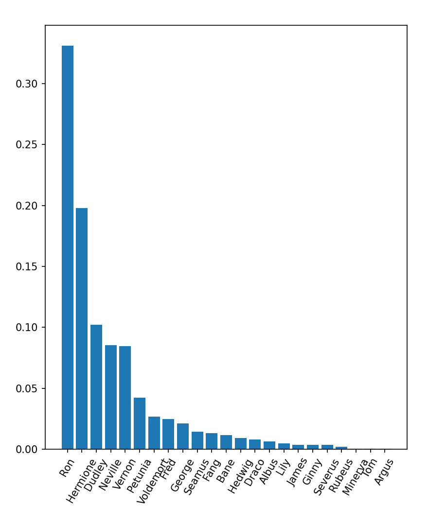
I won’t go over all the details about how I used matlabplot here, but instead focus on what the data is communicating. Seems like Ron is second popular to Harry (if Harry was in this graph). This makes sense since he is a frequently used side character in the series. The same can be said for Hermione as well. Using this graph, we should expect Ron to use less bits in its encoding with Argus using more considering Argus’s name is not used often.

Now that we can clearly see how often these names appear in the book Harry Potter and the Sorcerer’s Stone (the movie refers to the stone as the Philosopher’s versus the book where it is the Sorcerer’s stone), we can now perform Huffman encoding in the function perform_huffman_coding(...)

1
2
3
4
5
6
7
8
9
10
11
12
13
14
15
16
17
18
19
20
21
22
23
24
25
26
27
28
29
30
31
32
33
34
35
36
37
...

class FreqDistTracker:
    ...
    def convert_to_huffman_leaf_nodes(self):
        huffmanNodeList = []
        for i in range(len(self.probs)):
            huffmanNodeList.append(HuffmanNode(self.names[i], self.probs[i]))
        return huffmanNodeList
    ...

...

class HuffmanNode:
    def __init__(self, symbol, probabilitySum):
        self.symbol = symbol
        self.probabilitySum = probabilitySum
        self.left = None 
        self.right = None

    def set_left(self, left):
        self.left = left

    def set_right(self, right):
        self.right = right

...

def perform_huffman_coding(descendingFreqDistributionTracker):
    huffmanLeafNodes = descendingFreqDistributionTracker.convert_to_huffman_leaf_nodes()
    huffmanTree = build_huffman_encoding_tree(huffmanLeafNodes)
    print_huffman_encodings(huffmanTree[0], "")
    graph_huffman_tree(huffmanTree[0])

    return

...

With the variable descendingFreqDistributionTracker, I call the class function convert_to_huffman_leaf_nodes(...) to convert each individual probability and name into a HuffmanNode. This is to create and store the initial leaf nodes of the binary tree that will make up our Huffman encodings.

With the initial leaf nodes stored in huffmanLeafNodes, I begin building the Huffman tree. This is done in the function build_huffman_encoding_tree(...) til I end up with the root/parent of the tree which is stored in the list variable huffmanTree.

The functions print_huffman_encodings(...) and graph_huffman_tree(...) will end up printing our encodings in console and provide a visual graph for our binary tree with tools matplotlib and networkx. Before we see what the console and visual graph look like, lets see how we end up building the Huffman tree in build_huffman_encoding_tree(...)

1
2
3
4
5
6
7
8
9
10
11
12
13
14
15
16
17
18
19
20
21
...

def build_huffman_encoding_tree(huffmanTree):
    while len(huffmanTree) != 1:
        leftNode = huffmanTree.pop()
        rightNode = huffmanTree.pop()

        newProbabilitySum = leftNode.probabilitySum + rightNode.probabilitySum
        newParentNode = HuffmanNode(str(newProbabilitySum), newProbabilitySum)
        newParentNode.left = leftNode
        newParentNode.right = rightNode

        index = huffmanTree.__len__() - 1
        while index >= 0 and huffmanTree[index].probabilitySum < newParentNode.probabilitySum:
            index = index - 1

        huffmanTree.insert(index + 1, newParentNode)

    return huffmanTree

...

The end goal for building a huffman tree is that we end up with a root HuffmanNode in the variable huffmanTree. This is what len(huffmanTree) != 1 checks as we loop through the list, creating and assigning references between HuffmanNode’s.

But wait, why would we pop the last two elements in the list with huffmanTree.pop() when assigning our leftNode and rightNode? In the visual graph showing a huffman encoding step by step, we see the lowest probable elements are not always found at the end. This is different in the code, as huffmanTree starts off in descending order. This means the lowest probable elements will always be found at the end of the list, hence I pop the last two elements.

We then calculate the newProbabilitySum and store it in a newParentNode with references back to the leftNode and rightNode. This creates a new parent that can be referenced as a larger probability.

But for this newParentNode to be used, we need to insert it into huffmanTree. And not just insert it anywhere, but where the newProbabilitySum will not break the descending order present in huffmanTree. This is what the while loop accomplishes on line 14, as it checks two things:

If we reached the end of the list with index >= 0
When we found a higher probability than newProbabilitySum

When we found the proper index for the newParentNode to be placed at, we then record it with the index variable. This index variable is then used to perform the insertion with huffmanTree.insert(index + 1, newParentNode).

We then continue this process until the root is found. This ends up building the Huffman Tree. At that, it is time to see the encodings produced for each character and its visual representations.

Philosophers Stone Entropy, Encodings, and Visual Graph

******************************* Philosophers Stone Data *******************************
Entropy of characters from "Philosophers Stone": 3.0973347772966444
Binary for Symbol Petunia with probability 4.23% is: 0000
Binary for Symbol George with probability 2.12% is: 00010
Binary for Symbol Lily with probability 0.51% is: 0001100
Binary for Symbol Albus with probability 0.66% is: 0001101
Binary for Symbol Bane with probability 1.17% is: 000111
Binary for Symbol Dudley with probability 10.21% is: 001
Binary for Symbol Hermione with probability 19.77% is: 01
Binary for Symbol Fred with probability 2.48% is: 10000
Binary for Symbol Voldemort with probability 2.7% is: 10001
Binary for Symbol Fang with probability 1.31% is: 100100
Binary for Symbol Seamus with probability 1.46% is: 100101
Binary for Symbol Severus with probability 0.36% is: 10011000
Binary for Symbol Ginny with probability 0.36% is: 10011001
Binary for Symbol James with probability 0.36% is: 10011010
Binary for Symbol Minerva with probability 0.07% is: 1001101100
Binary for Symbol Argus with probability 0.07% is: 10011011010
Binary for Symbol Tom with probability 0.07% is: 10011011011
Binary for Symbol Rubeus with probability 0.22% is: 100110111
Binary for Symbol Draco with probability 0.8% is: 1001110
Binary for Symbol Hedwig with probability 0.95% is: 1001111
Binary for Symbol Vernon with probability 8.46% is: 1010
Binary for Symbol Neville with probability 8.53% is: 1011
Binary for Symbol Ron with probability 33.11% is: 11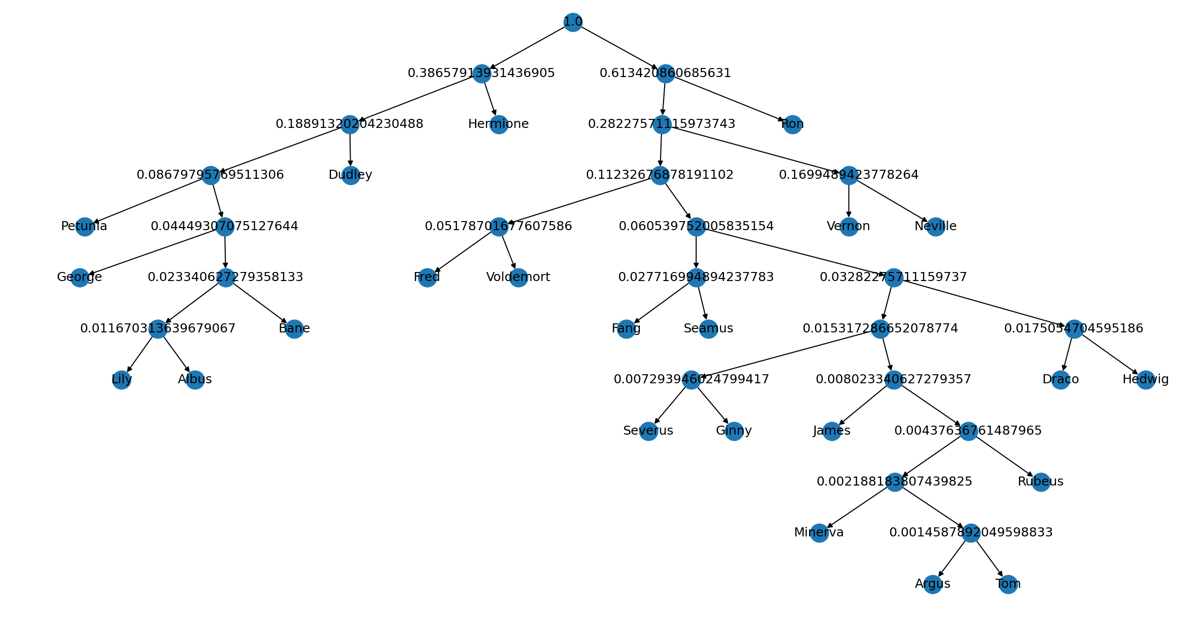

Chamber of Secrets Entropy, Encodings, and Visual Graph

******************************* Chamber of Secrets Data *******************************
Entropy of characters from "Chamber of Secrets": 3.4036128885897714
Binary for Symbol Hermione with probability 16.3% is: 00
Binary for Symbol Vernon with probability 2.08% is: 01000
Binary for Symbol Tom with probability 1.12% is: 010010
Binary for Symbol Voldemort with probability 1.22% is: 010011
Binary for Symbol George with probability 4.62% is: 0101
Binary for Symbol Fred with probability 5.23% is: 0110
Binary for Symbol Fang with probability 1.42% is: 011100
Binary for Symbol Rubeus with probability 0.15% is: 011101000
Binary for Symbol Minerva with probability 0.2% is: 011101001
Binary for Symbol Albus with probability 0.36% is: 01110101
Binary for Symbol Mason with probability 0.76% is: 0111011
Binary for Symbol Lucius with probability 1.47% is: 011110
Binary for Symbol Petunia with probability 1.47% is: 011111
Binary for Symbol Ginny with probability 5.94% is: 1000
Binary for Symbol Neville with probability 1.52% is: 100100
Binary for Symbol Draco with probability 1.73% is: 100101
Binary for Symbol Myrtle with probability 3.4% is: 10011
Binary for Symbol Dudley with probability 1.78% is: 101000
Binary for Symbol Gilderoy with probability 1.83% is: 101001
Binary for Symbol Seamus with probability 0.91% is: 1010100
Binary for Symbol Aragog with probability 0.96% is: 1010101
Binary for Symbol Argus with probability 0.41% is: 10101100
Binary for Symbol Severus with probability 0.3% is: 101011010
Binary for Symbol Molly with probability 0.3% is: 101011011
Binary for Symbol Hedwig with probability 1.02% is: 1010111
Binary for Symbol Dobby with probability 7.67% is: 1011
Binary for Symbol Ron with probability 35.8% is: 11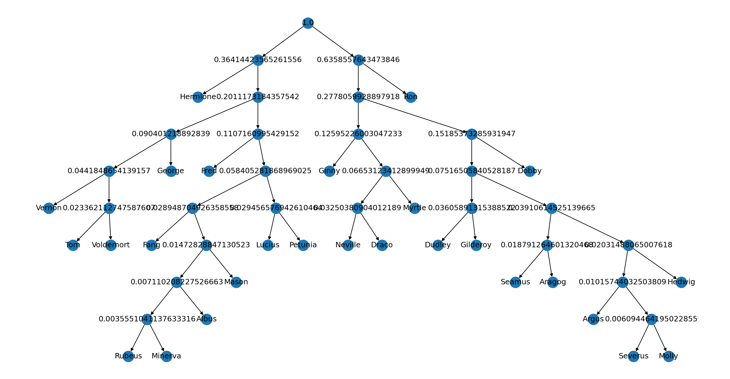

Do excuse on how messy the binary tree graphs look as I had trouble styling these

So what can we take away from these graphs and encodings. The first observation you could take away is there is more information stored in the book Chamber of Secrets with an entropy value of 3.4036 bits versus Philosophers Stone that has an entropy value of 3.0973. This may be due to more characters being present in the Philosophers Stone.

Another cool observation is to see the small bit encodings coming with high percentages. For example, take Ron who has the percentages 35.8% and 33.11%. Both encodings came out to be 11 due to it being a frequently used character name (he had the highest percentage of all). Now take Minerva who has the percentages 0.07% and 0.2%. Considering this character is not as relevant as other characters, the encodings turned out to be longer and different with 011101001 and 1001101100 being produced. The takeaway is: The more the use, the smaller the encoding!

It is also nice to see the visual graphs are showing the data in a way that is easily understood through observation. You can tell higher probabilities will be closer to the root while lower probabilities end up further away.

With the graphs, entropy value, and bits printed, this completely demonstrates the power of Huffman encodings. Through probability, you can turn complex symbols into its simplest form of 1’s and 0’s, effectively communicating the same information! Including the entropy value, this can give a clear indicator of the amount of surprise expected when encoding a set of symbols.

Checkpoint

In this post, I demonstrated how simple counting can lead to complex methods of information extraction. A small portion was also dedicated to Claude Shannon as his contributions made a new field of innovation that has much relevance today. The methods discussed included calculating the total amount of surprise that can be expected (Entropy) and converting symbols into 0’s and 1’s (Shannon Fano and Huffman). With these tools available, you gain more with less as storing and sharing information becomes easier while also gaining an expectation of its final result. I also walked through a coding example of Huffman encoding with its entropy value displayed for two books of Harry Potter. I think learning about these encoding methods was interesting and taught me a lot about how information theory works overall. I hope to explore more on the different ways you can use entropy to gain more information on what you are examining in future as well. The coding for this portion was also frustrating as much as it was rewarding as small logical errors always found a way past me. Through each correction however, I learned a new lesson, and that is the greatest reward.